“History Doesn’t Repeat Itself, but It Often Rhymes” — Mark Twain
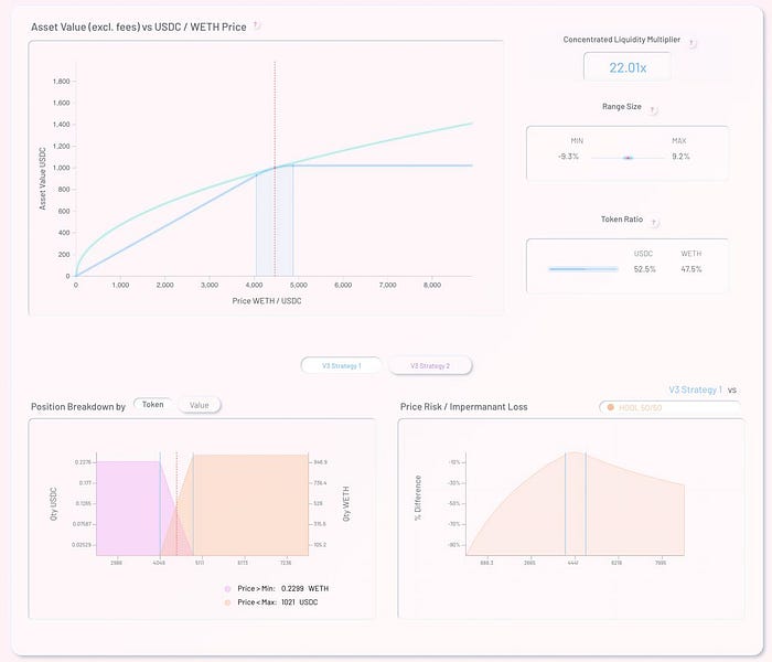
Defi-Lab Uniswap V3 simulator was born as a tool to support Uniswap Liquidity Providers in the process of designing their LP strategies and to highlight the risk and rewards linked to providing concentrated liquidity in Uniswap V3.
The success of any Uniswap LP position depends on two fundamental components:
- Impermanent loss: risk of losing money due to a divergence between the price at which we deposit our funds and the price at the moment we close our position
- Fees generated by the trading supported by the pool
Our goal is to help users understand and simulate the impact of these two components and help estimate possible results.
Impermanent loss can be clearly explained mathematically and we provide several visualisations to support our users simulating the effect of changing prices on their investments.

Fees generated, on the contrary, are highly uncertain; we can’t create exact models to determine the amount of fees that a pool will generate in the future but we can help our users supporting a simulation based on historical data of LP positions to support their analysis and their decisions.
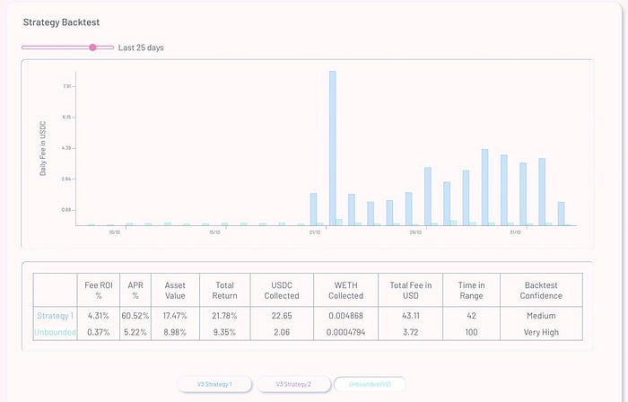
We expanded our tool to give the possibility to users to calculate historical performances of Uniswap LP strategies based on a new approach

A new approach to Uniswap V3 pool Backtesting
Uniswap LP strategy are highly differentiated, each investor can select its own range of active liquidity and each one will collect fee differently.
To backtest a strategy we therefore need to collect data and compute the specific conditions of the strategy under exam.
1. Extract Historical Data for a specific Uniswap V3 tool
To support our analysis we need to collect historical data about the Uniswap V3 pool in consideration. We use TheGraph PoolHourData subgraph for this matter.
As described in the Uniswap V3 white paper, for each pool Uniswap contracts are tracking the total amount of fees (fg) that would have been earned by 1 unit of unbounded liquidity that was deposited when the contract was first initialised. Unbounded liquidity can be easily described as a strategy that provides liquidity to the entire price range (MinLimit = 0 , MaxLimit = ∞ ).
We can calculate the fee earned by 1 unit of unbounded liquidity in one period as following:
F_Unb = fg(t) — fg(t-1)
2. Define position to be tested
In order to determine the historical fee of an LP position we need to first calculate the amount of liquidity an LP is providing. Liquidity is a function of the strategy (MinLimit and MaxLimit) and the initial investment
Liquidity = LiquidityFunction(MinLimit, MaxLimit, investment)
For our calculations we need also to determine the liquidity the same investment would generate if we would select an unbounded strategy.
LiquidityUnb = LiquidityFunction(0, ∞, investment)
3. Historical fee calculation
At the beginning of each period a LP can either:
a) Provide liquidity to the entire range, and in this case the fee earned can be easily determined:
MyFeeUnb = F_unb * LiquidityUnb
b) Provide concentrated liquidity to a specific range. The fee in this case are determined by the time the price spends in the active liquidity range and by the multiplier (as described here: https://uniswap.org/blog/uniswap-v3/ )
MyFee = MyFeeUnb * Multiplier * Time spent in Range
However the multiplier can be expressed as following:
Multiplier = Liquidity / LiquidityUnb
Therefore we can rewrite the previous formula as:
MyFee = F_Unb * Liquidity * Time spent in Range
And finally calculate the historical fee as MyFee earned in each period under analysis.
This sounds good, but does it actually work?
The theory is fun (kind of..), but does it actually work?
We backtested the backtester against more than 500 existing currently open in Uniswap v3 with the following results

When the the position is active for around 100% of the time the backtest is extremely precise, when the time in range is lower the precision decreases.
This is due to the approximation we need to apply when calculating the time spent in range parameter. Using TheGraph hourly data we can’t determine precisely the amount of time the price spent in the range but only an approximation.
Conclusions
This new functionality will allow fast and reliable backtesting directly within our simulator.
Past performances are not a guarantee of future results but they represent an important base of analysis and a support in our LP strategy definition.
